Chapter 3 Linear Mixed Models
In Richard McElreath’s book “Statistical Rethinking”, chapters 13 and 14 deal with multilevel models. In Gelman’s Book, see ” Part 2A: Multilevel Models” and the following.
One very graspable introduction to LMMs is this video.
We have already come across a Linear Mixed Model (LMM)
in the first chapter, where we used the rethinking and lme4 packages to fit a model with
random intercepts to determine our
Intraclass Correlation Coefficients (ICCs).
The are called random intercept since they are drawn from a common normal distribution,
of which the parameters (mean and standard deviation) are estimated from the data.
The main reason for using LMMs is that they allow us to model data with hierarchical structure, such as repeated measures (of the same subject) or nested data (math scores in different schools within different school districts).
For example, in our Peter and Mary data set where they measured ROMs, we had two measurements per subject. The two measurements are clustered within the subject. They are not independent. Hence, the classical linear regression model is not appropriate and would lead to smaller standard errors.
Another example is our RESOLVE trial. We are conducting a cluster randomized trial (CRT) with \(20\) clusters (physiotherapy offices) and over \(200\) patients. Measurements within a cluster could be correlated (more similar compared to other clusters). One could also think of the physiotherapists performing the treatments as clusters, since - potentially - the outcomes for all their patients could be correlated due to a more similiar treatment from the same therapists compared to others. Here the outcome measures are nested within the physiotherapists which are nested within the physiotherapy offices (assuming they only work for one office).
3.1 Example: Reed Frog tadpole mortality - two levels
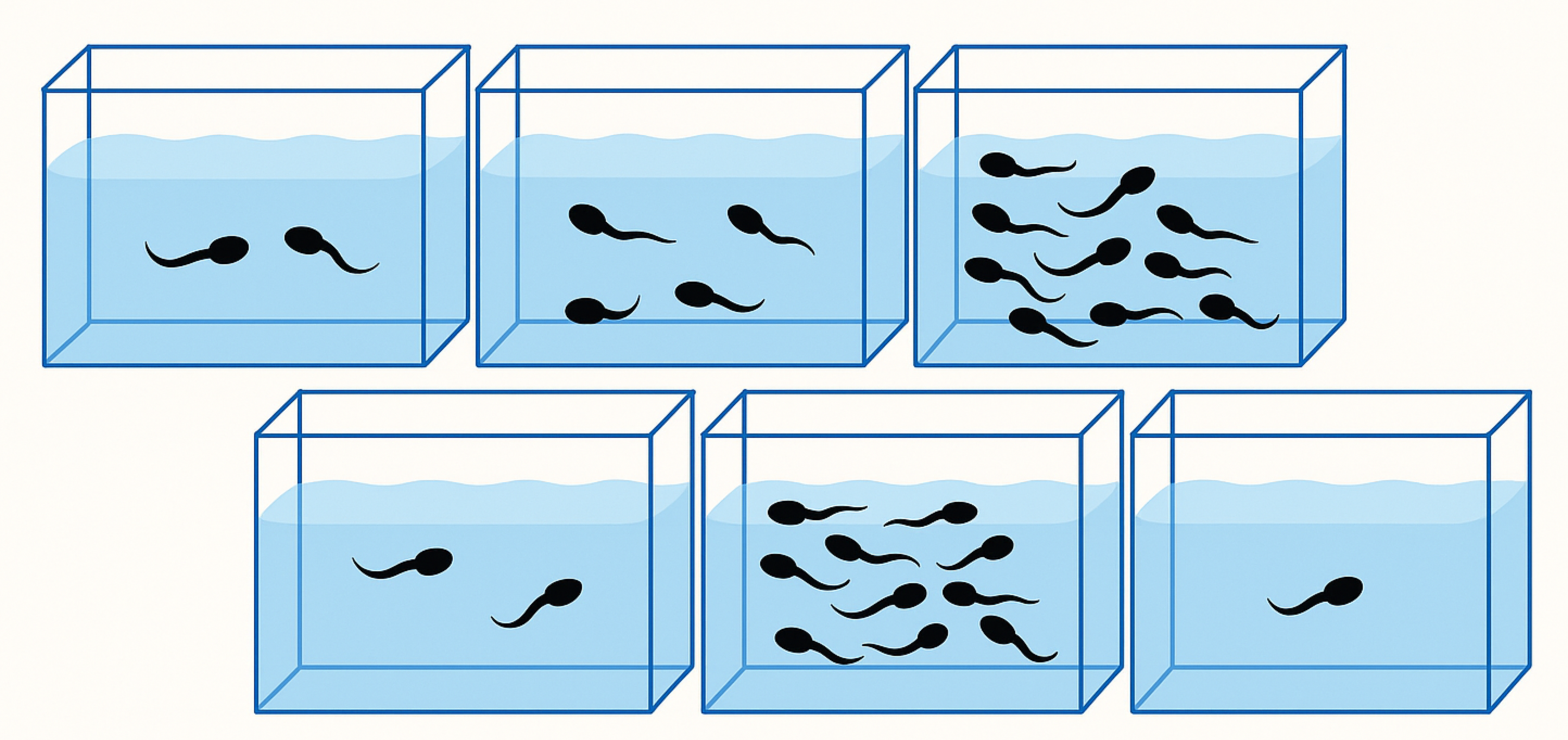
Let’s start with Example 13.1 from McElreath’s book (p.401) (Tadpoles in tanks, image by GPT4o).
## 'data.frame':    48 obs. of  5 variables:
##  $ density : int  10 10 10 10 10 10 10 10 10 10 ...
##  $ pred    : Factor w/ 2 levels "no","pred": 1 1 1 1 1 1 1 1 2 2 ...
##  $ size    : Factor w/ 2 levels "big","small": 1 1 1 1 2 2 2 2 1 1 ...
##  $ surv    : int  9 10 7 10 9 9 10 9 4 9 ...
##  $ propsurv: num  0.9 1 0.7 1 0.9 0.9 1 0.9 0.4 0.9 ...
Variables are explained here (see also p.401 in the book). The original paper can be found here.
The number of surviving tadpoles surv should be modeled. Now, each row is a different “tank” (\(48\) in total), an experimental environment that contains tadpoles. Obviously, the tanks are one option for clustering the data, assuming the tadpoles within the same tank live in a more similar environment than those in different tanks (or get a more similiar “treatment”). We could rewrite the data set to have one row per individual tadpole (instead of number of survived a binary variable) and the cluster variable called tank (exercise 1). We would then model the survival of each individual tadpole (\(1\) could mean survived and \(0\) could mean died). Formally, this would be a so-called logistic regression, since our outcome is binary (survided/died).
When estimating the number of surviving tadpoles we could consider the following options:
- Complete pooling (exercise 6): Estimate the overall survival probability (ignoring the tank effect). In this case, one might miss between-variance from the different tanks. A single intercept is used for all tanks.
- No pooling: Estimate the survival probability for each tank (ignoring the overall effect completely). Here, the tanks do not “know” anything from one another. Information of one tank is not used for the other tanks. An intercept is estimated for each tank (\(48\) in total). This approach would be equivalent to using indicator variables for each tank.
- Partial pooling: Estimate the survival probability for each tank, but use information from the other tanks.
3.1.1 Model 13.1. Partial pooling using regularizing priors
Let’s start with the second model (intercept for each tank) with a regularizing prior. We want to model the number of surviving tadpoles in the tanks by using a binomial distribution with different survival probabilities for each tank.
Here is our model in the typical notation:
\[ \begin{array}{rcl} S_i &\sim& Binomial(N_i, p_i) \\ logit(p) &=& \alpha_{TANK}[i] \\ \alpha_j &\sim& \text{Normal}(0, 1.5)~\text{for } j=1,\ldots,48 \end{array} \]
This is a varying intercept model (the simplest kind of varying effects model) with \(48\) intercepts (one for each tank).
The number of surviving tadpoles \(S_i\) in tank \(i\) is modeled as a binomial distribution with \(N_i\) trials (the number of tadpoles in the tank) and \(p_i\) the survival probability of tank \(i\). The regularizing prior for \(\alpha_j\) is a normal distribution with mean \(0\) and standard deviation \(1.5\).
Technically, we could use different priors for each intercept, but this would be a bit cumbersome and we do not have useful prior information about the survival probabilities of the tanks.
Notice that we use a logit link function to transform the probability \(p\) (range \((0,1)\))
to the range \((-\infty, \infty)\).
This way, we can use a normal distribution for the prior of the intercepts.
The inverse of the logit function is also available in rethinking: inv_logit.
rethinking::inv_logit(0)gives the probability of \(0.5\). So, we assume a coin flip for
the survival probability of the tadpoles in the tanks a priori
(maybe not the worst starting point if you have no clue).
What survaival probabilities do we assume a priori? Well, according to the normal distribution with a standard deviation of \(1.5\) we assume that the 95% of the logit-transformed survival probabilities are between \(-3\) and \(3\). This means that the survival probabilities in the tanks are in:
## [1] 0.04742587 0.95257413This assumption seems rather reasonable and survival probabilities are not constrained very much.
Next we define the data set for the model and use the ulam function
from the rethinking package to fit the model.
library(rethinking)

d$tank <- 1:nrow(d)
dat <- list(S = d$surv,
            N = d$density,
            tank = d$tank)

# approximate posterior
set.seed(122)
m13.1 <- ulam(
  alist(
    S ~ dbinom(N, p),
    logit(p) <- a[tank],
    a[tank] ~ dnorm(0, 1.5)
  ) , data = dat,
  chains = 4,
  log_lik = TRUE,
  cores = detectCores() - 1)
## Running MCMC with 4 chains, at most 7 in parallel, with 1 thread(s) per chain...
##
## Chain 1 Iteration: 1 / 1000 [ 0%] (Warmup)
## Chain 1 Iteration: 100 / 1000 [ 10%] (Warmup)
## Chain 1 Iteration: 200 / 1000 [ 20%] (Warmup)
## Chain 1 Iteration: 300 / 1000 [ 30%] (Warmup)
## Chain 1 Iteration: 400 / 1000 [ 40%] (Warmup)
## Chain 1 Iteration: 500 / 1000 [ 50%] (Warmup)
## Chain 1 Iteration: 501 / 1000 [ 50%] (Sampling)
## Chain 1 Iteration: 600 / 1000 [ 60%] (Sampling)
## Chain 1 Iteration: 700 / 1000 [ 70%] (Sampling)
## Chain 1 Iteration: 800 / 1000 [ 80%] (Sampling)
## Chain 1 Iteration: 900 / 1000 [ 90%] (Sampling)
## Chain 1 Iteration: 1000 / 1000 [100%] (Sampling)
## Chain 2 Iteration: 1 / 1000 [ 0%] (Warmup)
## Chain 2 Iteration: 100 / 1000 [ 10%] (Warmup)
## Chain 2 Iteration: 200 / 1000 [ 20%] (Warmup)
## Chain 2 Iteration: 300 / 1000 [ 30%] (Warmup)
## Chain 2 Iteration: 400 / 1000 [ 40%] (Warmup)
## Chain 2 Iteration: 500 / 1000 [ 50%] (Warmup)
## Chain 2 Iteration: 501 / 1000 [ 50%] (Sampling)
## Chain 2 Iteration: 600 / 1000 [ 60%] (Sampling)
## Chain 2 Iteration: 700 / 1000 [ 70%] (Sampling)
## Chain 2 Iteration: 800 / 1000 [ 80%] (Sampling)
## Chain 2 Iteration: 900 / 1000 [ 90%] (Sampling)
## Chain 2 Iteration: 1000 / 1000 [100%] (Sampling)
## Chain 3 Iteration: 1 / 1000 [ 0%] (Warmup)
## Chain 3 Iteration: 100 / 1000 [ 10%] (Warmup)
## Chain 3 Iteration: 200 / 1000 [ 20%] (Warmup)
## Chain 3 Iteration: 300 / 1000 [ 30%] (Warmup)
## Chain 3 Iteration: 400 / 1000 [ 40%] (Warmup)
## Chain 3 Iteration: 500 / 1000 [ 50%] (Warmup)
## Chain 3 Iteration: 501 / 1000 [ 50%] (Sampling)
## Chain 3 Iteration: 600 / 1000 [ 60%] (Sampling)
## Chain 3 Iteration: 700 / 1000 [ 70%] (Sampling)
## Chain 3 Iteration: 800 / 1000 [ 80%] (Sampling)
## Chain 3 Iteration: 900 / 1000 [ 90%] (Sampling)
## Chain 3 Iteration: 1000 / 1000 [100%] (Sampling)
## Chain 4 Iteration: 1 / 1000 [ 0%] (Warmup)
## Chain 4 Iteration: 100 / 1000 [ 10%] (Warmup)
## Chain 4 Iteration: 200 / 1000 [ 20%] (Warmup)
## Chain 4 Iteration: 300 / 1000 [ 30%] (Warmup)
## Chain 4 Iteration: 400 / 1000 [ 40%] (Warmup)
## Chain 4 Iteration: 500 / 1000 [ 50%] (Warmup)
## Chain 4 Iteration: 501 / 1000 [ 50%] (Sampling)
## Chain 4 Iteration: 600 / 1000 [ 60%] (Sampling)
## Chain 4 Iteration: 700 / 1000 [ 70%] (Sampling)
## Chain 4 Iteration: 800 / 1000 [ 80%] (Sampling)
## Chain 4 Iteration: 900 / 1000 [ 90%] (Sampling)
## Chain 4 Iteration: 1000 / 1000 [100%] (Sampling)
## Chain 1 finished in 0.1 seconds.
## Chain 2 finished in 0.1 seconds.
## Chain 3 finished in 0.1 seconds.
## Chain 4 finished in 0.1 seconds.
##
## All 4 chains finished successfully.
## Mean chain execution time: 0.1 seconds.
## Total execution time: 0.2 seconds.## mean sd 5.5% 94.5% rhat ess_bulk
## a[1] 1.717154006 0.7747045 0.54616751 3.00284170 1.0000687 3842.501
## a[2] 2.428617822 0.9211741 1.06824055 4.00015385 1.0012690 3260.212
## a[3] 0.752957586 0.6606081 -0.30096467 1.87725390 0.9994289 3657.926
## a[4] 2.392671596 0.9029471 1.04232310 3.96444320 0.9999341 4901.360
## a[5] 1.698600986 0.7501296 0.56599784 2.95760400 1.0010747 3583.085
## a[6] 1.709016626 0.7333373 0.61628599 2.93631575 1.0043948 3791.625
## a[7] 2.394662704 0.8967971 1.05357265 3.91037710 1.0021691 4633.411
## a[8] 1.751520527 0.8358778 0.51949731 3.11502600 1.0010314 2908.886
## a[9] -0.368916633 0.6263820 -1.40362045 0.63108741 1.0014184 5011.742
## a[10] 1.721989971 0.7876527 0.53971156 3.01818445 1.0064067 4743.990
## a[11] 0.762625202 0.6504815 -0.23379561 1.84594325 1.0042895 4356.338
## a[12] 0.360839662 0.6212530 -0.61653294 1.35696620 1.0003393 5427.338
## a[13] 0.747187659 0.6556836 -0.26629876 1.86578240 1.0047650 4965.966
## a[14] 0.004006226 0.6030814 -0.96596033 0.95626616 1.0015451 3860.382
## a[15] 1.698071502 0.7557423 0.58532612 3.00604665 1.0044770 4060.982
## a[16] 1.718281276 0.7589570 0.55788234 3.01417210 0.9995458 4085.653
## a[17] 2.540229640 0.6715384 1.51315760 3.67929090 1.0045229 3551.210
## a[18] 2.143608256 0.6099572 1.24664285 3.19176460 1.0027772 4601.028
## a[19] 1.814013282 0.5661173 0.96992496 2.74369310 1.0008102 3875.396
## a[20] 3.123650833 0.8415721 1.90725255 4.55287270 1.0001108 4325.296
## a[21] 2.144628056 0.6206063 1.21321885 3.18875240 1.0003712 4533.942
## a[22] 2.147574902 0.5862451 1.27518855 3.13301315 1.0054417 3115.241
## a[23] 2.158113205 0.6232680 1.23542735 3.20262840 1.0031826 4470.846
## a[24] 1.559385117 0.5054760 0.81471935 2.39450025 1.0050444 4677.140
## a[25] -1.100464102 0.4645629 -1.90970175 -0.37079074 1.0031187 4404.834
## a[26] 0.066658204 0.3997793 -0.57122361 0.71319580 1.0064293 5082.203
## a[27] -1.543870059 0.4969425 -2.35267600 -0.80927273 1.0049318 4888.677
## a[28] -0.545686639 0.3798291 -1.16412750 0.05957414 1.0141192 4539.855
## a[29] 0.076432999 0.3891808 -0.54687735 0.68588656 1.0063621 4372.045
## a[30] 1.317149701 0.4699257 0.61627877 2.10864310 1.0045814 4237.156
## a[31] -0.730232329 0.4142389 -1.41215210 -0.08699833 1.0056791 4674.458
## a[32] -0.380477602 0.3973004 -1.02838145 0.22966973 1.0027171 4757.953
## a[33] 2.854476850 0.6688006 1.86231770 3.93923980 1.0028748 4265.441
## a[34] 2.465178502 0.6016136 1.57307340 3.49223990 1.0034665 4026.537
## a[35] 2.475988085 0.6001981 1.62509180 3.45605210 1.0022452 3520.649
## a[36] 1.906146592 0.4793998 1.17540695 2.69468780 1.0091406 3637.720
## a[37] 1.903268812 0.4848702 1.17045730 2.68925485 0.9999314 4580.692
## a[38] 3.377291100 0.7728682 2.21480150 4.70722490 0.9999677 3559.742
## a[39] 2.448119286 0.5794139 1.58287005 3.42906255 1.0005167 4544.304
## a[40] 2.154826607 0.5110004 1.38358250 3.05123950 1.0057481 3928.734
## a[41] -1.924960111 0.4805039 -2.72391445 -1.20680920 1.0003669 3217.189
## a[42] -0.639489130 0.3594361 -1.20374385 -0.07755664 1.0036102 3891.702
## a[43] -0.515434665 0.3438150 -1.06684055 0.01709138 1.0067069 3206.309
## a[44] -0.399514162 0.3554107 -0.97334898 0.16487656 1.0043647 5212.318
## a[45] 0.519393681 0.3592609 -0.05772033 1.08264245 1.0022088 4807.785
## a[46] -0.636130179 0.3468987 -1.20742535 -0.10853365 1.0071298 3963.335
## a[47] 1.919195782 0.4916630 1.16999095 2.74101715 1.0000987 3428.411
## a[48] -0.061061407 0.3286406 -0.57313044 0.45005764 1.0009603 3435.612## [1] 0.8477619The R-output from precis(m13.1, depth = 2)shows the posterior means and standard deviations of
our \(48\) interecepts (\(48\) tanks with tadpoles). These intercepts are on the scale \((-\infty, \infty)\).
Note that you can always switch from the range \((-\infty, \infty)\) to a probability using the logistic function
from the rethinking package - these functions are called squashing functions for a reason.
The inv_logitfunction does the same.
\[ \mathrm{logistic}(x) = \mathrm{inv\_logit}(x) = \frac{1}{1 + e^{-x}} \]
The other way around works as well, using the logit function.
\[\text{logit}(p) = \log\left( \frac{p}{1 - p} \right)\]
Let’s quickly see if these are indeed inverse functions of each other -> exercise 5.
3.1.2 Model 13.2: Partial pooling using adaptive pooling
Next, we use adaptive pooling. For this, we use priors for the a[tank] parameters.
This model learns from the data how much the intercepts should be pulled towards a common mean.
Now we have an additional level in the model hierarchy:
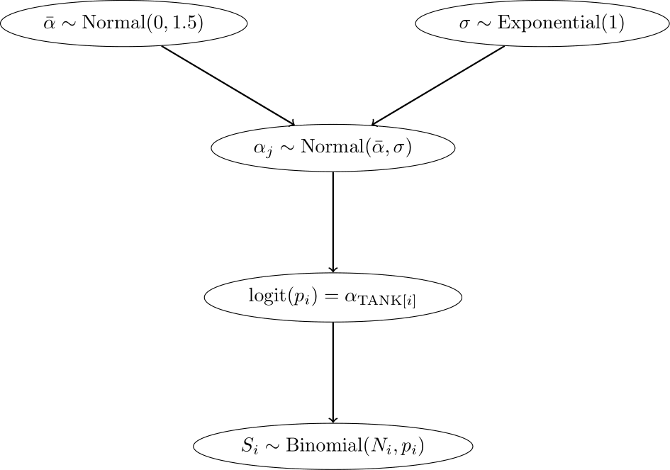
- In the top level, the outcome is \(S\), the parameters are the intercepts \(\alpha_{TANK[i]}\), and the priors are \(\alpha_j \sim N(\bar{\alpha}, \sigma)\).
- In the second level, the “outcome” are the intercepts \(\alpha_{TANK[i]}\), the parameters are \(\bar{\alpha}\) and \(\sigma\), and the priors are \(\bar{\alpha} \sim N(0, 1.5)\) and \(\sigma \sim \text{Exponential}(1)\).
\[ \begin{array}{rcl} S_i &\sim& \text{Binomial}(N_i, p_i) \\ \text{logit}(p) &=& \alpha_{\text{TANK}[i]} \\ \alpha_j &\sim& \text{Normal}(\bar{\alpha}, \sigma)\\ \bar{\alpha} &\sim& \text{Normal}(0, 1.5)\\ \sigma &\sim& \text{Exponential}(1) \end{array} \]
Since the parameters in the prior of the \(\alpha_j\) have also priors (last two lines are new), we have a multilevel model. In this case, we have two levels and the parameters \(\bar{\alpha}\) and \(\sigma\) are called hyperparameters. The priors of the hyperparameters are called hyperpriors. The amount or regularization is controlled by the hyperparameter \(\sigma\) and is learned from the data. \(\sigma\) controls, how much the intercepts are allowed to deviate from the mean \(\bar{\alpha}\). The smaller \(\sigma\), the more the intercepts are pulled towards the mean \(\bar{\alpha}\).
Below, we see the model hierarchy:
We now fit the model using the ulam function from the rethinking package.
## [conflicted] Will prefer posterior::var over any other package.## [conflicted] Removing existing preference.
## [conflicted] Will prefer posterior::sd over any other package.m13.2 <- ulam(
alist(
S ~ dbinom(N, p),
logit(p) <- a[tank],
a[tank] ~ dnorm(a_bar, sigma),
a_bar ~ dnorm(0, 1.5),
sigma ~ dexp(1)
) , data = dat,
chains = 4,
log_lik = TRUE,
cores = detectCores() - 1)## Running MCMC with 4 chains, at most 7 in parallel, with 1 thread(s) per chain...
##
## Chain 1 Iteration: 1 / 1000 [ 0%] (Warmup)
## Chain 1 Iteration: 100 / 1000 [ 10%] (Warmup)
## Chain 1 Iteration: 200 / 1000 [ 20%] (Warmup)
## Chain 1 Iteration: 300 / 1000 [ 30%] (Warmup)
## Chain 1 Iteration: 400 / 1000 [ 40%] (Warmup)
## Chain 1 Iteration: 500 / 1000 [ 50%] (Warmup)
## Chain 1 Iteration: 501 / 1000 [ 50%] (Sampling)
## Chain 1 Iteration: 600 / 1000 [ 60%] (Sampling)
## Chain 1 Iteration: 700 / 1000 [ 70%] (Sampling)
## Chain 1 Iteration: 800 / 1000 [ 80%] (Sampling)
## Chain 1 Iteration: 900 / 1000 [ 90%] (Sampling)
## Chain 1 Iteration: 1000 / 1000 [100%] (Sampling)
## Chain 2 Iteration: 1 / 1000 [ 0%] (Warmup)
## Chain 2 Iteration: 100 / 1000 [ 10%] (Warmup)
## Chain 2 Iteration: 200 / 1000 [ 20%] (Warmup)
## Chain 2 Iteration: 300 / 1000 [ 30%] (Warmup)
## Chain 2 Iteration: 400 / 1000 [ 40%] (Warmup)
## Chain 2 Iteration: 500 / 1000 [ 50%] (Warmup)
## Chain 2 Iteration: 501 / 1000 [ 50%] (Sampling)
## Chain 2 Iteration: 600 / 1000 [ 60%] (Sampling)
## Chain 2 Iteration: 700 / 1000 [ 70%] (Sampling)
## Chain 2 Iteration: 800 / 1000 [ 80%] (Sampling)
## Chain 2 Iteration: 900 / 1000 [ 90%] (Sampling)
## Chain 2 Iteration: 1000 / 1000 [100%] (Sampling)
## Chain 3 Iteration: 1 / 1000 [ 0%] (Warmup)
## Chain 3 Iteration: 100 / 1000 [ 10%] (Warmup)
## Chain 3 Iteration: 200 / 1000 [ 20%] (Warmup)
## Chain 3 Iteration: 300 / 1000 [ 30%] (Warmup)
## Chain 3 Iteration: 400 / 1000 [ 40%] (Warmup)
## Chain 3 Iteration: 500 / 1000 [ 50%] (Warmup)
## Chain 3 Iteration: 501 / 1000 [ 50%] (Sampling)
## Chain 3 Iteration: 600 / 1000 [ 60%] (Sampling)
## Chain 3 Iteration: 700 / 1000 [ 70%] (Sampling)
## Chain 3 Iteration: 800 / 1000 [ 80%] (Sampling)
## Chain 3 Iteration: 900 / 1000 [ 90%] (Sampling)
## Chain 3 Iteration: 1000 / 1000 [100%] (Sampling)
## Chain 4 Iteration: 1 / 1000 [ 0%] (Warmup)
## Chain 4 Iteration: 100 / 1000 [ 10%] (Warmup)
## Chain 4 Iteration: 200 / 1000 [ 20%] (Warmup)
## Chain 4 Iteration: 300 / 1000 [ 30%] (Warmup)
## Chain 4 Iteration: 400 / 1000 [ 40%] (Warmup)
## Chain 4 Iteration: 500 / 1000 [ 50%] (Warmup)
## Chain 4 Iteration: 501 / 1000 [ 50%] (Sampling)
## Chain 4 Iteration: 600 / 1000 [ 60%] (Sampling)
## Chain 4 Iteration: 700 / 1000 [ 70%] (Sampling)
## Chain 4 Iteration: 800 / 1000 [ 80%] (Sampling)
## Chain 4 Iteration: 900 / 1000 [ 90%] (Sampling)
## Chain 4 Iteration: 1000 / 1000 [100%] (Sampling)## Chain 4 Informational Message: The current Metropolis proposal is about to be rejected because of the following issue:
## Chain 4 Exception: normal_lpdf: Scale parameter is 0, but must be positive! (in '/var/folders/pm/jd6n6gj10371_bml1gh8sc5w0000gn/T/RtmpRPKbBi/model-b56a7e1c28b0.stan', line 15, column 4 to column 32)
## Chain 4 If this warning occurs sporadically, such as for highly constrained variable types like covariance matrices, then the sampler is fine,
## Chain 4 but if this warning occurs often then your model may be either severely ill-conditioned or misspecified.
## Chain 4## Chain 1 finished in 0.1 seconds.
## Chain 2 finished in 0.1 seconds.
## Chain 3 finished in 0.1 seconds.
## Chain 4 finished in 0.1 seconds.
##
## All 4 chains finished successfully.
## Mean chain execution time: 0.1 seconds.
## Total execution time: 0.2 seconds.## mean sd 5.5% 94.5% rhat ess_bulk
## a[1] 2.1360104954 0.8661191 0.83424198 3.553682700 1.0026805 3270.394
## a[2] 3.0781335085 1.1236851 1.43096300 4.984337950 1.0021514 3333.772
## a[3] 1.0172166998 0.6728834 0.02487391 2.122557100 1.0017997 4433.035
## a[4] 3.0539084560 1.0673010 1.45577985 4.862345550 0.9991935 3292.307
## a[5] 2.1460704153 0.8885053 0.82128835 3.632871100 1.0012996 3243.212
## a[6] 2.1295681940 0.8491091 0.88580128 3.547453050 1.0068927 4014.260
## a[7] 3.0995747675 1.1423048 1.49656170 5.081114500 1.0000324 2876.988
## a[8] 2.1399446424 0.9003458 0.81845163 3.682066500 1.0014370 3989.652
## a[9] -0.1714730123 0.6191399 -1.18887420 0.817493905 1.0011313 3485.167
## a[10] 2.0975422705 0.8315647 0.86475233 3.491159800 1.0003507 3475.655
## a[11] 0.9972846111 0.6886670 -0.06780398 2.108900800 1.0035689 6346.111
## a[12] 0.5808274429 0.6321307 -0.39005998 1.589965800 1.0073548 4009.231
## a[13] 1.0044482950 0.6869233 -0.06659326 2.145820400 1.0062364 5228.172
## a[14] 0.1943572393 0.5958137 -0.75088828 1.137035850 1.0090229 4741.338
## a[15] 2.1509188614 0.8679934 0.90383891 3.653387850 1.0031940 3312.879
## a[16] 2.1333640552 0.9017144 0.80812878 3.653567300 1.0126010 4233.256
## a[17] 2.9192000930 0.8415071 1.68621300 4.328422500 1.0040634 4410.077
## a[18] 2.3925664980 0.6551941 1.42167145 3.513079150 1.0056149 4144.799
## a[19] 2.0077513930 0.5900888 1.11100110 2.993477400 1.0059627 3633.662
## a[20] 3.6725677750 1.0278681 2.20375370 5.475839300 1.0049323 3236.751
## a[21] 2.4059350610 0.6759614 1.38493480 3.559096600 1.0015502 5132.563
## a[22] 2.4065305525 0.6796675 1.42094305 3.541692650 0.9991290 3831.139
## a[23] 2.3861532095 0.6514720 1.42360935 3.472103550 1.0043729 4128.680
## a[24] 1.7089185740 0.5393019 0.87925440 2.627249950 1.0048578 4608.699
## a[25] -1.0120972883 0.4472418 -1.73198540 -0.326257340 1.0014661 4734.657
## a[26] 0.1608543317 0.3886832 -0.46547174 0.767354565 1.0023246 4941.014
## a[27] -1.4196695957 0.4932724 -2.25709745 -0.685836175 1.0028562 4123.586
## a[28] -0.4766474294 0.4060361 -1.14774660 0.151370735 1.0052220 3931.755
## a[29] 0.1694769825 0.4170077 -0.49255198 0.859140040 1.0020527 4739.882
## a[30] 1.4511140548 0.5133738 0.66183801 2.306309700 1.0011993 4978.641
## a[31] -0.6385969972 0.4191422 -1.30238420 0.002327188 1.0021641 4600.143
## a[32] -0.3101703440 0.3728743 -0.90309567 0.287795040 0.9998292 5387.376
## a[33] 3.1774488200 0.7655335 2.08349505 4.549344000 1.0049724 3861.331
## a[34] 2.7053424900 0.6559522 1.73698945 3.801545200 1.0012059 4418.032
## a[35] 2.7221132200 0.6273888 1.81337830 3.780182650 1.0009124 3645.004
## a[36] 2.0546272795 0.4965714 1.31339900 2.878739800 1.0062188 4941.400
## a[37] 2.0584841305 0.5188968 1.26758275 2.917035500 1.0015659 4474.923
## a[38] 3.8972652500 0.9072140 2.63982515 5.508591850 1.0012459 3004.701
## a[39] 2.6974989445 0.6268090 1.74492005 3.751004950 0.9991983 3801.943
## a[40] 2.3462939655 0.5804959 1.47061030 3.318163350 1.0087612 3756.208
## a[41] -1.8135897265 0.4813845 -2.60774680 -1.085182300 1.0000863 3538.261
## a[42] -0.5797062286 0.3540843 -1.15873190 -0.026373790 1.0025961 3932.502
## a[43] -0.4553320681 0.3423639 -1.00197960 0.080289540 1.0064972 4788.740
## a[44] -0.3294683952 0.3311178 -0.86400261 0.191963110 1.0099484 4098.959
## a[45] 0.5781168532 0.3537311 0.02023151 1.152294850 1.0051871 4534.473
## a[46] -0.5734202532 0.3340746 -1.11167870 -0.052582168 1.0045535 3855.996
## a[47] 2.0729423255 0.5180042 1.30783735 2.935491000 1.0033394 3591.954
## a[48] -0.0003544386 0.3378852 -0.52970810 0.533022400 1.0060391 4423.905
## a_bar 1.3420237045 0.2527708 0.94567161 1.760416550 1.0011880 2994.562
## sigma 1.6149891850 0.2052025 1.30750950 1.961327050 0.9998544 1674.452Now, the output of precis(m13.2, depth = 2) additionally shows the posterior means
and standard deviations of the hyperparameters \(\bar{\alpha}\) (a_bar)
and \(\sigma\) (sigma).
3.1.3 Conceptual difference between model 13.1 and 13.2
Model 13.1 is not a multilevel model, we just tell the model there are \(48\) tanks and each tank has its own intercept. For each intercept, we use the same prior distribution (\(Normal (0, 1.5)\)), but we could use different ones if we had knowledge about the survival probabilities of some of the tanks. Note that the priors themselves are not connected via another level. They do their thing independently.
By decreasing the variance of these priors, we are dampening the influence of the data on the intercepts which are drawn towards to overall mean.
Increasing the variance of the priors to a value large enough will result in the raw survival probabilities for each tank. This would be the same as if we took indicator variables for each tank. See exercise 2.
Model 13.2 is a multilevel model. Now the model learns from the data from which overall mean and variance the intercepts are drawn (\(Normal(\bar{\alpha}, \sigma)\)). The prior for \(\bar{\alpha}\) expresses our belief about the mean survival probability, while the prior for \(\sigma\) expresses our belief about the variability of the survival probabilities.
Figure 13.1 from the book depicts the pooling effect of model 13.2. with respect to tadpole tank size.
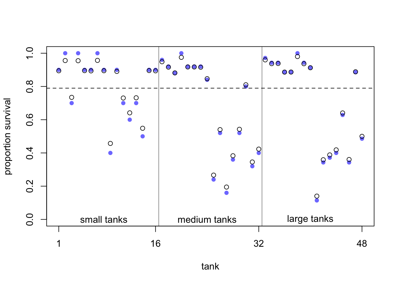
In exercise 2 we make the difference between the models 13.1 and 2 clearer. Figure 13.1 from the book shows the posterior survival probabilities for each tank from model 13.2 (black circles) and raw survival probabilities (blue filled points). What we can see is that the estimated survival probabilities for the hierarchical model are drawn towards the mean overall survival probability across all tanks (dashed line; \(logistic(\bar{\alpha}) \approx 0.79\)).
- In large tanks, there is less shrinkage (enough information/observations), while in small tanks the estimates are pulled more towards the mean (information is used from other tanks).
- The more extreme the raw survival probability (with respect to the overall survival probability), the more it is pulled towards the mean.
This is the pooling effect of the model. The phenomenon is called shrinkage.
See also exercise 3 to improve your understanding of two models.
3.1.4 Compare models 13.1 and 13.2 with respect to predictive ability on unseen data
In QM2 we talked about the difference between explanatory vs. predictive models. If you are interested, you can read section 7.4 (p.217) in the book.
In a prediciton context we ask ourselves: How well do the models predict the data (which was measured using residuals \(y_i - \hat{y}_i\) in regression)?
There are many nuances but the main paradigm (also in classical machine learning) is to fit the model on a training set and evaluate the model on a test set. Should you be interested in the (admittedly very technical) details, I can recommend the book Elements of Statistical Learning by Hastie, Tibshirani and Friedman (free here).
During training, the model tries to learn the underlying structure of the data. The test set is used to evaluate the model’s performance on unseen data. This is the ultimate and brutally honest test of the model’s predictive ability.
For instance, if you think back to our body height prediction example in QM2, we would fit the model on 80% of people (training set) and see how precise the model is on the remaining 20% of people (test set). Let’s do this in exercise 7.
Remember, in prediction we do not care about interpretability of the model. We could have a blackbox model (e.g. neural networks) and still be happy with it. This performance can often be surprisingly good (like in the case of hand digit recognition reaching error rates as low as 0.09%), or surprisingly bad (when trying to predict some binary outcome using logistic regression in applied health research where the performance is often not far away from the base rate probability).
In order to estimate the predictive ability of a model, there are many criteria available. One of them is the WAIC:
##       WAIC      lppd  penalty  std_err
## 1 216.2614 -81.72813 26.40257 4.679153## WAIC lppd penalty std_err
## 1 200.3715 -79.18461 21.00113 7.205089## WAIC SE dWAIC dSE pWAIC weight
## m13.2 200.3715 7.205089 0.00000 NA 21.00113 0.9996456832
## m13.1 216.2614 4.679153 15.88993 3.798405 26.40257 0.0003543168WAIC stands for Widely Applicable Information Criterion and is a measure of prediction accuracy on new data (out of sample deviance); see p.219 and p.404 in Statistical Rethinking. As it is pointed out in the book “Using tools like PSIS and WAIC is much easier than understanding them.”
We do not go into the details of WAIC, but as a first dirty rule of thumb, the model with the lower WAIC is preferred. One should never solely rely on this criterion, especially not if one is interested in causal questions.
What are the columns?
WAIC: guess of the out-of-sample deviance.SE: standard error of the WAIC estimate.dWAIC: difference of each WAIC from the best model (with the smallest WAIC).dSE: standard error of this difference. Here, the standard error of the difference (\(3.79\)) is much smaller compared to the difference in WAIC between the models (\(15.88993\)). Here, one can distinguish between the models using WAIC. \(\rightarrow\) m13.2 is preferred (with respect to predictive ability on unseen data).pWAIC: prediction penalty. This is close to the number of parameters in the posterior.weight: the Akaike weight, a measure of relative support for each model. In our case, it is almost 1 for model 13.2 and almost 0 for model 13.1.
Feel free to read p.227 in the book, specifically before you use WAIC in a publication or thesis.
One can also plot this information for a better overview:
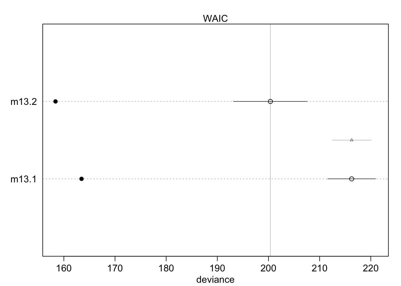
The filled points show how the model performs on the data it was trained on. Typically, this is lower compared to the out-of-sample deviance (open points) for both models. Section 13.2 (especially Figure 13.3.) in the book shows that partial pooling also yields (on average) better predictions compared to no pooling, it’s a tradeoff between over- and underfitting.
3.1.4.1 Frequentist version model 13.2
In the Frequentist setting we can use the lme4 package to fit the analog
to model 13.2. To be more specific,
we use a generalized linear mixed model (GLMM).
Generalized because we assume a binomial distribution for the response variable,
while usually we have a continuous outcome variable (like body height in cm).
Let’s fit the model and explain the outcome first. \(S\) is the number of surviving tadpoles, \(N\) is the number of tadpoles in the tank.
library(lme4)

m_lmer <- glmer(
  cbind(S, N - S) ~ (1 | tank),
  data = dat,
  family = binomial(link = "logit"),
  control = glmerControl(optimizer = "bobyqa")
)
summary(m_lmer)
## Generalized linear mixed model fit by maximum likelihood (Laplace
## Approximation) [glmerMod]
## Family: binomial ( logit )
## Formula: cbind(S, N - S) ~ (1 | tank)
## Data: dat
## Control: glmerControl(optimizer = "bobyqa")
##
## AIC BIC logLik -2*log(L) df.resid
## 271.6 275.3 -133.8 267.6 46
##
## Scaled residuals:
## Min 1Q Median 3Q Max
## -0.5981 -0.2255 0.1267 0.2457 0.9677
##
## Random effects:
## Groups Name Variance Std.Dev.
## tank (Intercept) 2.459 1.568
## Number of obs: 48, groups: tank, 48
##
## Fixed effects:
## Estimate Std. Error z value Pr(>|z|)
## (Intercept) 1.3786 0.2505 5.503 3.74e-08 ***
## ---
## Signif. codes: 0 '***' 0.001 '**' 0.01 '*' 0.05 '.' 0.1 ' ' 1For convergence reasons (after trial and error), we used the bobyqa optimizer.
We do not care so much about the technical details behind the model fitting procedure.
Briefly, the model is not fitted using the least squares method anymore,
but the maximum likelihood method
(see also Westfall p.43-52),
which is another way of finding model parameters in parametric statistics.
Interestingly, the way to fit the model in front of us is outlined in the help file of the command
glmer (see ?glmer).
The syntax (1 | tank) means that we fit a random intercept for each tank.
For details on the random effect structure definition see
p.7 here.
You will always see such a term if you model clustered data in the Frequentist
setting (at least in R).
AIC (Akaike Information Criterion) and BIC (Bayesian Information Criterion) are two measures of model fit which both consider the model fit and the number of parameters simultaneously. Both punish the number of parameters in the model, but not equally strong.
In the summary output, we see the values for AIC, BIC and the log-likelihood.
The latter is used to fit the model. -2logLik is the so-called deviance of
the model and has - under \(H_0\) - a \(\chi^2\) distribution that can be exploited
for hypothesis testing. This term takes the place of the residual sum of squares
in least squares regression.
The Std.Dev. of the Random effect tank is \(1.568\) which schould be somewhat similar
to the sigma in the Bayesian model (\(1.614989185\)), which is the case here.
The major difference is that in the Frequentist model, this \(\sigma\) is only
learned from the data, while in the Bayesian model we have priors too.
The Fixed effect (Intercept) (\(1.3786\)) is the logit of the mean survival probability
across all tanks and analog to the a_bar (\(1.3420237045\)) in the Bayesian model.
df.residis \(46\), sample size is \(48\). Two degrees of freedom are lost due
to the estimation of the overall (Intercept) and the random effect (the standard
deviation \(\sigma\) of tank).
And of course, at the bottom of the summary output, for the stargazers among us, are the Signif. codes.
In summary, both (Frequentist and Bayesian) models deliver rather similar results.
We leave it as an exercise (4) to compare the model-estimated survival probabilities in the tanks for both models.
Section 13.2. in the book shows that partial pooling also yields (on average) better predictions compared to no pooling, it’s a tradeoff between over- and underfitting (i.e. the raw probabilities in each tank without knowledge of the other tanks and one overall survival probability that ignores differences between tanks completely).
3.2 Exercises
Solutions to the exercises can be found here.
3.2.1 Exercise 1
- Do some descriptive statistics on the data set reedfrogs.
- Use the
dplyrandtidyrpackages to create a new data set with one row per individual tadpole. For every tadpole, we want the variable surv_bin to be \(1\) if the tadpole survived and \(0\) if it died. - Feel free to check out the solution and ask a LLM (e.g., GPT) to explain the code - in this case it does a good job.
3.2.2 Exercise 2
We want to better undestand the pooling effect of model 13.2 vs. model 13.1.
- Calculate the mean survival probability for each tank in model 13.1/2. Use the function
logistic(or equivalentlyinv_logit) from therethinkingpackage to transform the \(48\) intercepts to probabilities. - Calculate the raw survival probability for each tank by dividing the number of surivals (S) by
the tank size (N). Or you can just use the column
propsurv, which is the same. - Plot the mean survival probability for each tank from model 13.1 against the raw survival probability. What do you see?
- Do the same for model 13.2. What do you see?
- In the model definition of 13.1 change the priors for the intercepts and
play with different large/small values for XX:
a[tank] ~ dnorm(0, XX). What do you see? - In the model definition of 13.2 change the priors for the intercepts and
play with different large/small values for XX:
a[tank] ~ dnorm(0, XX)and also the prior for \(\sigma\) (which regulates the pooling):sigma ~ dexp(XX).
3.2.3 Exercise 3
We want to check the correlation of the posterior estimates of the intercepts (a[tank]) for model 13.1 and 2.
- Use the
extract.samplesfunction to extract the posterior samples of the intercepts. - Use the
corfunction to calculate the correlation between the first \(2\) intercepts for both models. - Is there a correlation of the posterior samples for
a[1]anda[2]in either model? - Reason about the results.
3.2.4 Exercise 4
Go back to the Frequentist version of the tadpole model 13.2 above.
- Calculate and compare the model-estimated survival probabilities in the tanks for both models (Frequentist and and Bayesian model 13.2).
- What would be the Frequentist equivalent of model 13.1? Compare the model-estimated survival probabilities again.
3.2.5 Exercise 5
- Verify with R that the
logitandlogistic(=inv_logit) functions are indeed inverse functions of each other. - Also plot both functions for clarity.
3.2.6 Exercise 6
Consider the tadpole data set again.
- Fit a model with complete pooling, i.e. one intercept for all tanks, without a regularizing prior.
Hence, the tanks to not “know” anything from one another. Use the
rethinkingpackage.
3.2.7 Exercise 7
Consider our regression model (\(\mu_i = \alpha + \beta_1 x_i + \beta_2 x_i^2\)) for the body height of the !Kung San people in QM2.
- Randomly select 80% of your obervations (rows in the data set).
- Fit the model again using the
rethinkingpackage on the 80% of observations. - Predict the body height of the remaining 20% of observations using the model.
- Calculate the root mean squared error (RMSE) of the predictions: \[ \text{RMSE} = \sqrt{\frac{1}{n}\sum_{i=1}^n (h_i - \hat{h}_i)^2}\] where \(h_i\) is the observed body height and \(\hat{h}_i\) is the predicted body height.
- Calculate the RMSE for the 80% of obervations as well and compare the two RMSEs. What do you oberve? Was this an accident?
- Repeat creating a training and test set and calculating the RMSE for both the training and the test set \(100\) times. Draw a histogram of the RMSEs for training and test set. What do you observe?
3.3 TODOS
- Create many practically relevant ICC examples
- Create many practically relevant validity examples
- Application movement detection with R/Python as example of machine learning/AI.
- AI Example, Claude and LEAN with Terence
- Examples of Reliability studies - eLearning?
- Last Chapter - Introduction to AI. Previous statistical analyses is a special case of neuronal networks.
- table 2 fallacy
- mention missing values, missingness mechanisms
- Chapter: Sample size calculations for multivariate regression, Proportions, ICCs, t.test
- AIC, BIC, cross-validation, Model selection (best subset, leaps….), Variable selection
- More on bias variance tradeoff, show for polynomial regression?
- Restrictive cubic splines?
- Causal inference, DAGs, counterfactuals
- Create final chapter with “topics we have not covered for time reasons: some known unknowns.”
Topics: Sample size calculations, missing data, composition data,
causal inference,…
Frequently asked master thesis questions:
- How to deal with missing data?
- How calculate the sample size for XX?