Chapter 2 Introduction
2.1 What is statistical modeling and what do we need this for?
Typically, one simplifies the complex reality (and loses information) in order to make it better understandable (explainable), mathematically treatable and to make predictions.
Underlying our models, there are theories which should be falsifiable and testable. For instance, I would be really surprised if I pull up my multimeter and measure the voltage (V) and electric current (I) at a resistance (R) in a circuit and find that Ohm’s law \(V = IR\) is not true. This law can be tested over and over again and if one would find a single valid counterexample, the law would be falsified. It is also true that the law is probably not 100% accurate, but an extremely precise approximation of reality. Real-world measurements carry measurement errors and when plotting the data, one would see that the data points might not lie exactly on a straight line. This is not a problem.
A statistical model is a mathematical framework that represents the relationships between variables, helping us understand, infer, and predict patterns in data. It acts as a bridge between observed data and the real-world processes that generated them. In health research, where variability and uncertainty are inherent, statistical models are valuable tools for making sense of complex phenomena. You can watch this as short intro.
In QM1 we have already made testable predictions with respect to the probability of an event. In our 1000-researcher experiment we stated for instance, that the probability of observing \(66\) or more findings would be very unlikely. If such an event would occur (while not repeating the experiment many times), we would reconsider our model. Inexactly, we could have stated something like: “We will not see more than 100 findings by chance.” With respect to our multiple choice test at the end of QM1 we could predict: “We will not see a single person answering all questions correctly by chance in our lifetime (given the frequency of tests).” Note, that in this context, the word predict is used with respect to a future event (chance finding or chance passing of the test). As we will see, there does not necessarily have to be a temporal connection in order to predict something.
Depending on the task at hand, we would use different models. In any case, logical reasoning and critical thinking comes first, then comes the model. It makes no sense to estimate statistical models just for the sake of it.
All models are wrong, but some are useful. Or to quote George Box:
“Since all models are wrong the scientist cannot obtain a ‘correct’ one by excessive elaboration. On the contrary following William of Occam he should seek an economical description of natural phenomena. Just as the ability to devise simple but evocative models is the signature of the great scientist so overelaboration and overparameterization is often the mark of mediocrity.”
In my opinion, statistical modeling is an art form: difficult and beautiful.
One goal of this course is to improve interpretation and limitations of statistical models. They are not magical tools turning data into truth. Firstly, the rule garbage in, garbage out (GABA) applies. Secondly, statistical models are based on data and their variability and have inherent limitations one cannot overcome even with the most sophisticated models. This is expressed for instance in the so-called bias-variance trade-off. You can’t have it all.
2.1.1 Explanatory vs. Predictive Models
I can recommend reading this article by Shmueli et al. (2010) on this topic.
Statistical models serve different purposes depending on the research question. Two primary goals are explanation and prediction, and each requires a different approach:
Explanatory models (the harder of the two) focus on understanding causal relationships. These models aim to uncover mechanisms and answer “why” questions. For example:
- Does smoking increase the risk of lung cancer? Yes. (If you want to see what a large effect-size looks like, check out this study.)
- How large is the effect (causal) of smoking on lung cancer? Large.
- Does pain education and graded sensorimotor relearning improve disability (a question we ask in our Resolve Swiss project)?
Explanatory models are theory-driven, designed to test hypotheses. Here, one wants to understand the underlying mechanisms and the relationships between variables and hence often uses (parsimonious) models that are more interpretable, like linear regression.
Predictive models prioritize forecasting/predicting (future) outcomes based on patterns in the data. These models aim to answer “what will happen?” For instance:
- Gait analysis using Machine Learning (ML)?
- Skin cancer detection using neural networks?
- If I know the age, sex and weight of a person, can I predict his/her height? Can I predict the height better with the given covariates compared to just guessing by using the mean height of my sample for the next patient?
Predictive models are data-driven, often using complex algorithms to achieve high accuracy. Their success is measured using metrics like Root Means Square Error (RMSE), Area Under the Curve (AUC), or prediction error on new, unseen data. Any amount of model complexity is allowed. One could for instance estimate a neural network (“just” another statistical model) with many hidden layers and neurons in order to improve prediction quality. Interpretability of the model weights is not a priority here.
While explanatory and predictive goals often complement each other, their differences highlight the importance of clearly defining the purpose of your analysis. In applied health research, explanatory models help identify causal mechanisms, while predictive models can guide real-world decisions by providing actionable forecasts. Together, they enhance both our understanding of phenomena and our ability to make informed decisions in complex environments.
2.1.2 Individual vs. Population Prediction
Another important distinction is between individual vs. population prediction. In the smoking example above, we can be very sure about the mean effects that smoking has on lung cancer. On an individual level, it is harder to predict the outcome. Nevertheless, individual predictions will be (notably) better than random guessing. We will discuss this in greater detail.
Statistical models are often much worse than one would naively expect, but they very often better than experts. If you are interested and want to boost your confidence in the predictive ability of statistical models, I recommend reading chapter 21 (“Intuitions vs. Formulas”) of Daniel Kahneman’s book “Thinking, Fast and Slow” (available in the ZHAW library). Of course, you should check if the studies mentioned in the book were replicated and if the results are still valid.
2.1.3 Practical Use of Statistical Models
In my opinion, we should never be afraid to test our statistical models (as honestly as possible) against reality. We could for instance ask ourselves:
“How much better does this model estimate an outcome than the arithmetic mean? (i.e., the linear model with just an intercept)”
“How much better does this model classify than random guessing?”
Is it worth the effort to collect data and estimate this model by using hundreds of hours of our time?
In some cases, these questions can be answered straightforwardly.
In advertising (Google, Facebook, …), a couple of percentage points in prediction quality might make a difference of millions of dollars in revenue offsetting the statisticians salary by a large margin.
Improved forecasts of a few percentage points in the stock market or just being slightly better than the average, will make you fabulously rich.
Improved cancer forecasting might save lives, money and pain and is of course not only measured in financial gains.
2.1.4 Start at the beginning
What do we actually want to do in general? Very broadly speaking we want to: describe the association of variables to each other that carry variability. Hence, the relationship is not deterministic like \[y = 2x + 3\] but rather we need to “loosen up” the relationship to account for variability (in \(x\) and \(y\)). So, \(y\) and \(x\) are not fixed but afflicted with uncertainty. Depending on your philosophical view, you might say you want to find the “true” but unknown relationship (here, \(2\) and \(3\) are the true coefficients) between variables. This is what we do in simulation studies all the time: We know the true relationship, simulate data by adding variability and then try to estimate the true relationship we assumed in the first place. This is an advantage the pioneers of statistics did not have. We can simulate millions of lines of data at the click of a button. For some practical applications, we can get a really nice and complete answer to our question (for instance sample size for proportions).
So we are looking for a function \(f\) such that
\[ \mathbf{Y} = f(\mathbf{X}) \]
where
- \(\mathbf{Y}\) is the “outcome”, “dependent variable” or “response”.
- \(\mathbf{X}\) are the “predictors”. \(\mathbf{X}\) can be a single Variable \(x\) or many variables \(x_1, x_2, \ldots, x_p\).
It is important to be aware of the notation here: “Predict” does not necessarily mean that we can predict the value in the future. It merely means we estimate the value (or mean) of \(Y\) given \(X\).
- This can be done at the same time points, known as cross-sectional analysis (“What is the maximum jumping height of a person given their age at a certain point in time, whereas both variables are measured at the same time?”);
- or at different time points, known as longitudinal analysis (“What is the maximum jumping height of a person 10 years later (\(t_2\)) given their baseline health status at time \(t_1\)?”).
The simplest statistical model would be the mean model where \(Y\) is “predicted” by a constant: \(Y = c\) which (at least in the classical linear regression) turns out to be \(c = \bar{x}\). This simple model is often surprisingly good, or, to put it in other words, models with more complexity are often not that much better.
2.2 A (simple) model for adult body heights in the Bayesian framework
As repetition, read the parts about Bayes statistics from QM1 again to refresh your memory about the Bayesian framework.
It’s recommendable to read the beginning of the book Statistical rethinking (hint: the online-version of the book differs a bit from the paper-version) up until page 39 as well. We are not completely new to the topic of Bayes thanks to QM1. In the Bayesian setting we use (well argued for) prior knowledge about a parameter or effect and update this knowledge with new data.
We want to start building our first model right away.
Let’s begin with the example in Statistical rethinking using data from the !Kung San people.
## 'data.frame':    544 obs. of  4 variables:
##  $ height: num  152 140 137 157 145 ...
##  $ weight: num  47.8 36.5 31.9 53 41.3 ...
##  $ age   : num  63 63 65 41 51 35 32 27 19 54 ...
## $ male : int 1 0 0 1 0 1 0 1 0 1 ...We want to model the adult height of the !Kung San people using prior knowledge (about the Swiss population) and data.
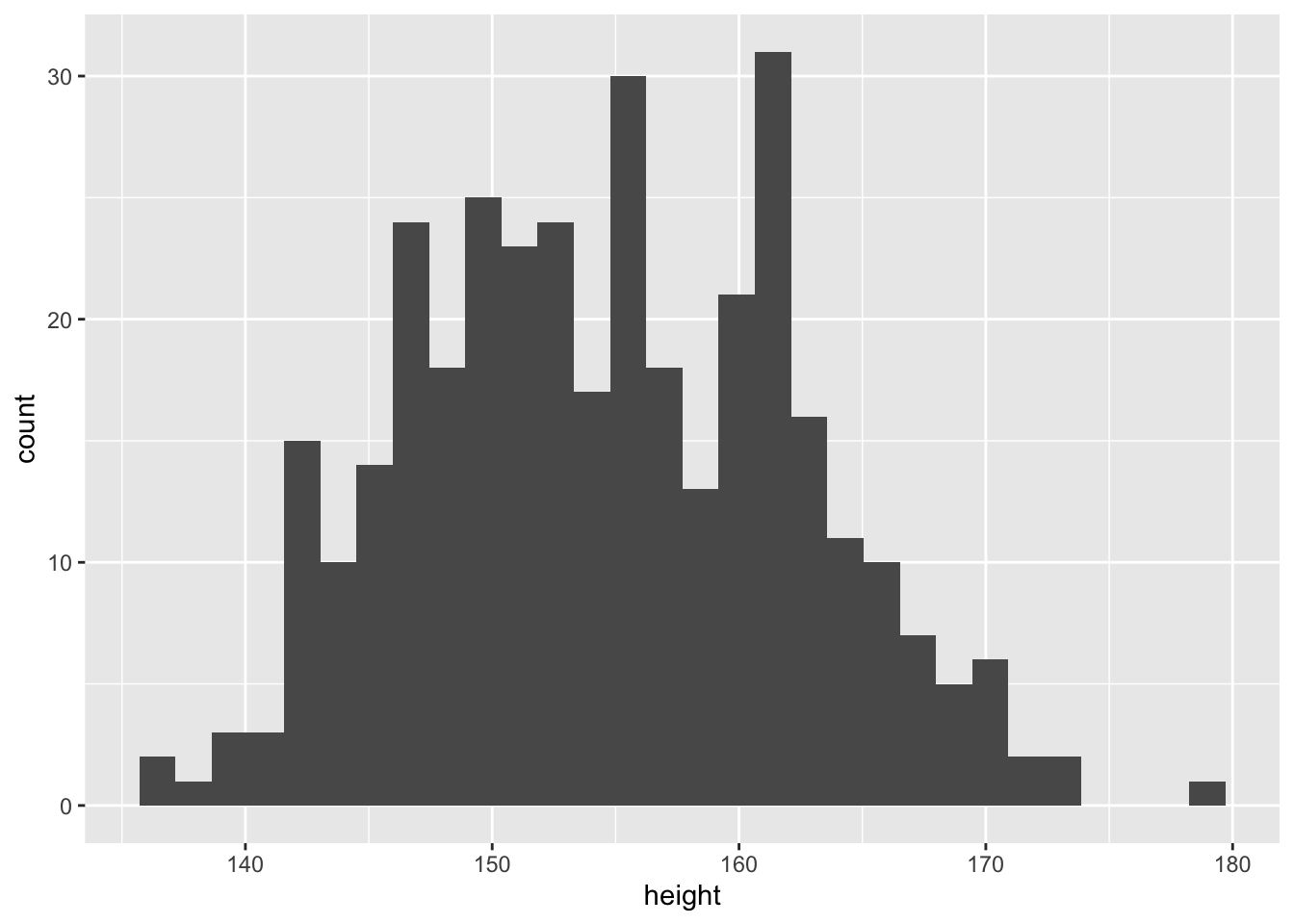
Since we already have domain knowledge in this area, we can say that heights are usually normally distributed, or at least a mixture of normal distributions (female/male). We assume the following model: \[h_i \sim \text{Normal}(\mu, \sigma)\]
As in QM1, we want to start with a Bayesian model and hence, we need some priors.
Since we are in Switzerland and just for fun, we use the mean of Swiss body heights as expected value for the prior for the mean. According to the link (Bundesamt für Statistik), the mean height of \(n=21,873\) people in the Swiss sample is \(171.1\) cm. We choose the same \(\sigma\) for the prior of the normal as in the book not to deviate too much from the example at hand.
Next comes our model definition in the Bayesian framework, which I often find more intuitive than the Frequentist approach:
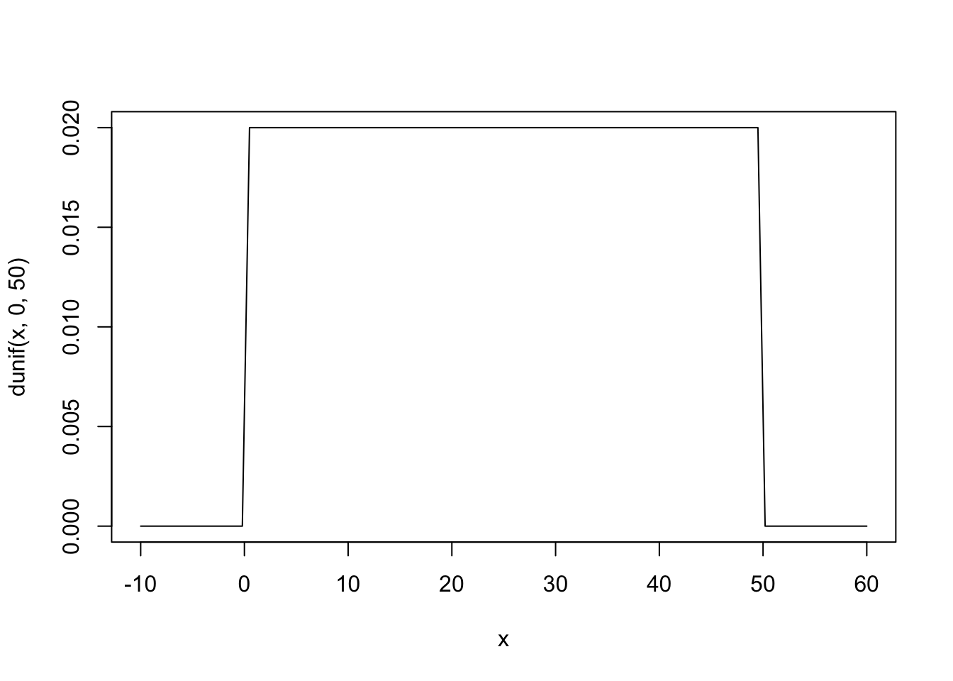
\[ h_i \sim \text{Normal}(\mu, \sigma) \] \[ \mu \sim \text{Normal}(171.1, 20) \] \[ \sigma \sim \text{Uniform}(0, 50) \]
Description of the model definition: The heights are normally distributed with unknown mean and standard deviation. As our current knowledge about the mean height, we use a prior distribution for the mean (we do not know but want to estimate) by assuming the mean of a population we know and a standard deviation of \(20\) cm which allows a rather large range of possible values for \(\mu\) (the unobserved population mean of the !Kung San people). \(\sigma\) (the unobserved standard deviation of the population of !Kung San people) is also unknown and a priori we restrict ourselves to values between \(0\) and \(50\) cm, whereas we assign equal plausibility to all values in this range (which can and should be critically discussed).
Visualisation of the model structure:
Mind that there is a conceptual difference between the normal distribution of the heights and the normal prior distribution of the mean. The latter expresses our prior knowledge/insecurity about the unobserved mean of the normal distribution of the heights. The normal distribution of the heights says we expect the heights to be normally distributed but we do not know the parameters (\(\mu\) and \(\sigma\)) yet. We will estimate these parameters using prior knowledge and the data.
Of course we would not need the prior here due to the large sample size, but let’s do it anyways for demonstration purposes. We are not completely uninformed about body heights and express our knowledge with the prior for \(\mu\). The \(20\) in the prior for the mean expresses our range of possible true mean values and acknowledge that there are a variety of different subpopulations with different means.
Using the Swiss data in the link one could estimate that the standard deviation of the heights from \(21,873\) Swiss people is around \(25.67\) cm (Exercise 1).
Remember, in the Bayesian world, there is no fixed but unknown parameter, but instead we define a distribution over the unobserved parameter.
We visualize the prior for \(\mu\):
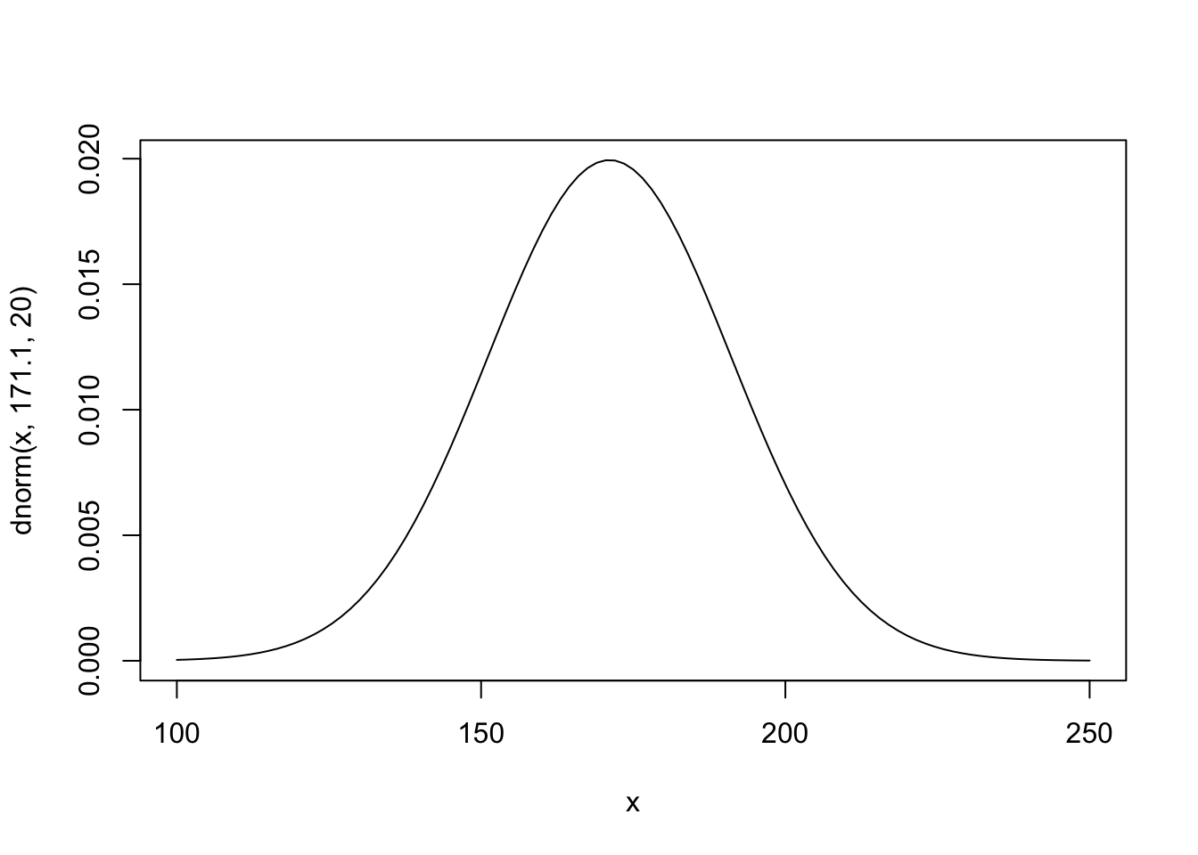
A wide range of population means is possible. One could discuss this distribution and maybe further restrict it.
The prior for \(\sigma\) is uniform between \(0\) and \(50\) cm. This is a very wide prior and just constrains the values to be positive and below \(50\) cm. This could be stronger of course.
Visualization of the prior for \(\sigma\):
Note, we didn’t specify a prior probability distribution of heights directly, but once we’ve chosen priors for \(\mu\) and \(\sigma\), these imply a prior distribution of individual heights.
Without even having seen the new data, we can check what our prior (model) for heights would predict. This is important. If the prior already predicts impossible values, we should reconsider our priors and/or model.
So, we simply draw \(\mu\) and \(\sigma\) from the priors and then draw heights from the normal distribution using the drawn parameters.
Visualisation of the prior for heights:
sample_mu <- rnorm(10^4, 171.1, 20)
sample_sigma <- runif(10^4, 0, 50)
prior_h <- rnorm(10^4, sample_mu, sample_sigma)
length(prior_h)
## [1] 10000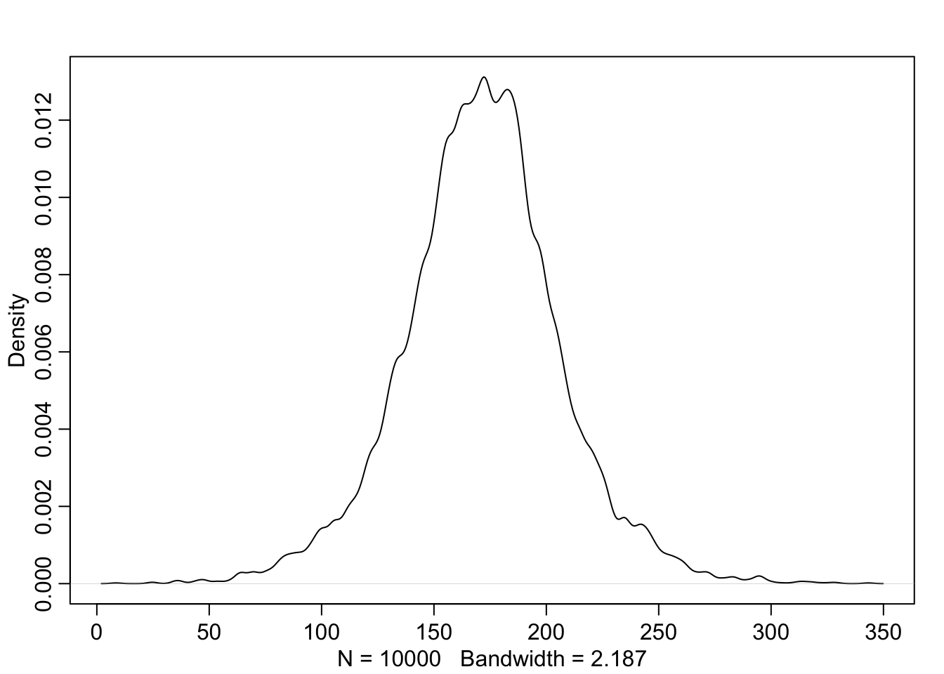
The prior is not itself a Gaussian distribution, but a distribution of relative plausibilities of different heights, before seeing the data.
Note how we have created the model predictions for heights. We first drew \(\mu\) and \(\sigma\) independently (there is no arrow between \(\mu\) and \(\sigma\)) from the priors. Then we drew heights from the normal distribution using the drawn parameters. You just follow the model structure.
Now, there are a couple of different ways to estimate the model incorporating the new data. For didactic reasons, grid approximation is often used (as in the books). For many parameters, this approach becomes more and more infeasible (due to combinatorial explosion).
We will skip that for now and use quadratic approximation instead which works well for many common procedures in applied statistics (like linear regression). Later, you’ll probably use (or the software in the background) mostly Markov chain Monte Carlo (MCMC) sampling to get the posterior. Pages 39 and the following explain the 3 concepts grid approximation, quadratic approximation and MCMC.
In short, quadratic approximation assumes that our posterior distribution of body heights can be approximated well by a normal distribution, at least near the peak.
Please read the addendum to get a clearer picture of what a bivariate normal distribution is.
Using the rethinking package we can estimate the model using quadratic approximation.
First, we define the model in the rethinking syntax (see R code 4.25 in the book).
library(rethinking)
flist <- alist(
  height ~ dnorm(mu, sigma),
  mu ~ dnorm(171.1, 20),
  sigma ~ dunif(0, 50)
)
Then we estimate/fit the model using quadratic approximation.
Now let’s take a look at the fitted model:
(Note: In the online-version of the book, they used the command map instead of quap.)
The precisfunction displays concise parameter estimate information
(from the posterior) for an existing model fit.
## mean sd 5.5% 94.5%
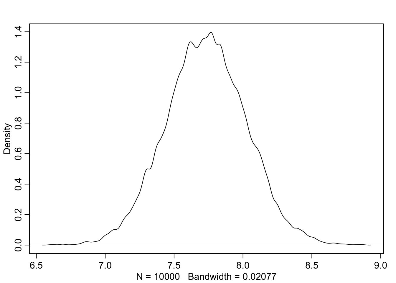
## mu 154.604922 0.4119789 153.946500 155.263344
## sigma 7.731042 0.2913585 7.265394 8.196689Above, we see the mean of the posterior for \(\mu\) and \(\sigma\); and a 89% credible interval for those parameters. Note that these are rather tight credible intervals. We are rather confident that the mean is somewhere between \(154\) and \(155\) cm and the standard deviation is between \(7\) and \(8\) cm.
We can now plot the posterior distribution of the mean (\(\mu\)) and the standard deviation (\(\sigma\)) separately by drawing from the posterior distribution.
##         mu    sigma
## 1 154.4525 8.001227
## 2 155.3379 7.909437
## 3 154.9235 7.693826
## 4 154.3972 8.026440
## 5 153.8498 8.386983
## 6 154.9913 7.853136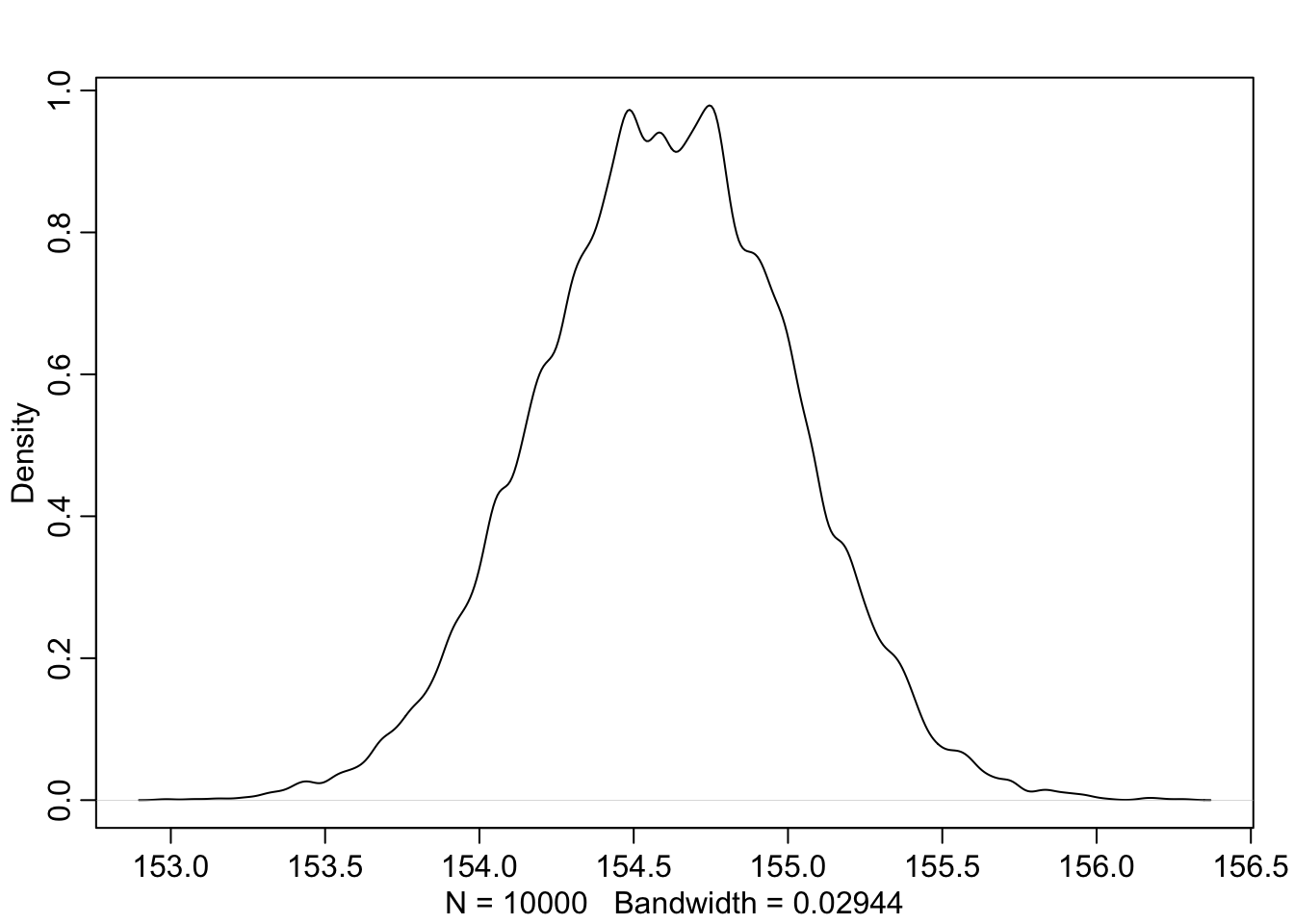
Note, that these samples come from a multi-dimensional posterior distribution. In our case, we approximated the joint posterior distribution of \(\mu\) and \(\sigma\) with a bivariate normal distribution. They are not necessarily independent from each other, but in this case they are (see exercise 6). We know this from the prior definition above. \(\mu\) and \(\sigma\) are both defined as normal respectively uniform distributions and by definition do not influence each other. This is also visible in the visualisation of the model structure: There is no confounding variable or connection between those priors. One could think of a common variable \(Z\) that influences both \(\mu\) and \(\sigma\). This could be genetic similarity which could influence both \(\mu\) and \(\sigma\).
Let’s verify that \(\mu\) and \(\sigma\) are uncorrelated:
##                 mu        sigma
## mu    0.1697265846 0.0001718597
## sigma 0.0001718597 0.0848897891
gives you the variance-covariance matrix of the parameters of the posterior distribution. In the diagonal you see the variance of the parameters.
##         mu      sigma
## 0.16972658 0.08488979
And we can compute the correlation matrix easily:
##                mu       sigma
## mu    1.000000000 0.001431763
## sigma 0.001431763 1.000000000
Let’s plot the posterior in 3D, because we can:
How beautiful is that?
This shows how credible each combination of \(\mu\) and \(\sigma\) is based on our priors and the data observed. The higher the mountain for a certain parameter combination, the more credible this combination is.
We see in the 3D plot, that the “mountain” is not rotated, indicating graphically that the parameters are independent from each other.
We also see in the correlation matrix, the correlation of the parameters is \(\sim 0\). In the context of a joint normal distribution, this means that the parameters are also independent.
And, it is not an accident that the posterior looks like this. Using quadratic approximation, we used the bivariate normal distribution to approximate the posterior.
2.3 Classical approach for the simplest model
We have seen, how we could use prior knowledge to fit a very simple model for body heights of a population (!Kung San) in the Bayesian framework.
Now, let’s start at the same point in the classical framework. Here, we do not use any prior knowledge, at least not that explicitly.
The classical approach to fit a regression line is the so-called least squares method.
There are hundreds of videos online explaining this method in great detail with animations. Maybe watch these videos later, when we add a predictor to the mean model, since most of instructional videos start at the simple linear regression using two parameters (intercept (\(\beta_0\) or \(\alpha\)) and slope (\(\beta_1\))).
The (simple mean-) model is:
\[ Y_i = height_i = c + \varepsilon_i \]
- for some \(c \in \mathbb{R}\) and
- normally distributed errors \(\varepsilon_i \sim \text{Normal}(0, \sigma)\).
The errors \(\varepsilon_i\) are on average zero and have a constant standard deviation of \(\sigma\). So, we assume there is a fixed, but unknown, constant \(c\) that we want to estimate and we assume that there is a special sort of error in our model that is normally distributed. Sometimes there is a large deviation from the true \(c\), sometimes there is a small deviation. On average, the deviations are zero and the errors should also be independent from each other: \[ \varepsilon_i \perp \varepsilon_j \text{ for } i \neq j\] This means that just because I have just observed a large deviation from the true \(c\) does not mean, that the probability of a large deviation in the next observation is higher/lower. Note, that we cannot readily define different types of errors in the classical framework.
But what is \(c\)? We determine the shape of the model ourselves (constant model, or mean model) and then estimate the parameter \(c\). By defining the shape of the model ourselves and imposing a distribution where we want to estimate the parameter of said distribution, we are in parametric statistics.
We choose the \(c\) which minimizes the sum of squared errors from the actual heights. This has the advantage that deviations upper and lower from the actual height are equally weighted. The larger the deviation the (quadratically) larger the penalty.
Why do we do that? Because, if the model assumptions (more on that later) are correct, the least squares estimator is a really good estimator. How good? Later…
We want to minimize the following function:
\[ SSE \text{ (Sum of Squared Errors) }(c) = (height_1 - c)^2 + (height_2 - c)^2 + \ldots + (height_n - c)^2 =\] \[ = \sum_{i=1}^{n} (height_i - c)^2\]
The SSE is a function of \(c\) and we want to find the \(c\) that minimizes the function. Since it is a quadratic function, we can always find the minimum. We have learnt in school how to do this (hopefully): Take the derivative of the function and set it to zero. Solve for \(c\) and you have the \(c\) which yields the minimum of SSE(c).
Let’s do that:
\[ \frac{d}{dc} SSE(c) = 2(height_1 - c)(-1) + 2(height_2 - c)(-1) + \ldots + 2(height_n - c)(-1) =\] \[ = -2 \sum_{i=1}^{n} (height_i - c)\]
This should be zero for the minimum: \[ -2 \sum_{i=1}^{n} (height_i - c) = 0\] \[ \sum_{i=1}^{n} (height_i - c) = 0\] \[ \sum_{i=1}^{n} height_i - n \cdot c = 0\] \[ \hat{c} = \frac{1}{n} \sum_{i=1}^{n} height_i = \overline{height_i}\]
The hat over the \(c\) indicates that this is the estimated value of the true but unknown \(c\). Every time we estimate a parameter, we put a hat over it.
And voilà, we have estimated the parameter \(c\) of the model, which is just the sample mean of all the heights. In contrast to before, we did not put in a lot of prior knowledge, but just estimated the parameter from the data.
In R, we can do this easily:
##
## Call:
## lm(formula = height ~ 1, data = d2)
##
## Residuals:
##      Min       1Q   Median       3Q      Max
## -18.0721  -6.0071  -0.2921   6.0579  24.4729
##
## Coefficients:
##             Estimate Std. Error t value Pr(>|t|)
## (Intercept) 154.5971     0.4127   374.6   <2e-16 ***
## ---
## Signif. codes:  0 '***' 0.001 '**' 0.01 '*' 0.05 '.' 0.1 ' ' 1
##
## Residual standard error: 7.742 on 351 degrees of freedom## [1] 352 4## [1] 154.5971## [1] 0.4126677## [1] 374.6285## [1] 7.742332The ~1 means that there is just a so-called intercept in the model.
There are no covariates, just the constant \(c\).
This is the simplest we can do. lm stands for linear model and with this base
command in R we ask the software to do the least squares estimation for us.
Let’s look at the R-output of the model estimation:
lm(formula = height ~ 1, data = d2): This is the model we estimated.Residuals: The difference between the actual height and the estimated height: \(r_i = height_i - \hat{c}\). A univariate 5-point summary is given.Coefficients: The estimated coefficients of the model. In this case, there is just the intercept. We get theStd. Errorof the estimate, i.e. the standard error (SE) of the mean, which is (according to the Central Limit Theorem) \[\frac{\sigma}{\sqrt{n}}\] and can be estimated by the sample standard deviation divided by the square root of the sample size. \(\hat{SE} = \frac{s}{\sqrt{n}}\)- the
t valueand thePr(>|t|)which is the \(p\)-value of the (Wald-)test of the null hypothesis that the coefficient is zero (\(H_0: \text{intercept}=0\)). This is a perfect example of an absolutely useless \(t\)-test. Why? Because obviously (exercise 2) the population mean of body heights is not zero.
Residual standard error: The standard deviation of the residuals \(r_i = height_i - \hat{c}\). In this case identical with the sample standard deviation of heights (exercise 3). \(351\) degrees of freedom. There are \(352\) observations and \(1\) parameter estimated (intercept/mean). Hence, there are \(352-1=351\) freely movable variables in the statistic of the sample standard deviation.
Let’s look at the situation graphically:
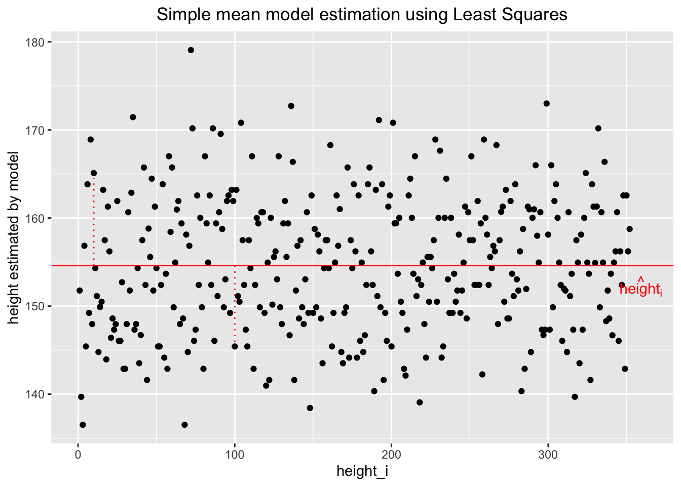
Above, the heights are plotted against the index of the observation (the order does not matter). The variability of heights around the regression line (constant in this case) seems to stay constant, which is a good sign. We will call this homoscedasticity later. The dashed vertical red lines show two residuals (one \(>0\), the other \(<0\)), the difference between the actual height and the estimated height. The model-estimated heights (\(\widehat{heights_i}\)) are all identical and nothing but the mean of all heights.
Peter Westfall explains in his excellent book a conditional distribution approach to regression, which is just what happens in the classical linear regression model. I highly recommend reading the first chapters.
What does this mean in this context? This means, that for every fixed value of the predictor (which we formally do not have), the distribution of the response is normal with mean \(\hat{c}\) and standard deviation \(\sigma\). Since, we do not have a predictor (apart from the intercept), we can say, that the distribution of the heights is normal with mean \(\hat{c}\) and standard deviation \(\sigma\). This is what we assumed in the model. It can also be directly seen in the formula:
\[ height_i = c + \varepsilon_i \]
If you add a normally distributed random variable (\(\varepsilon_i\)) to a constant (\(c\)), the result is a normally distributed. No surprise here.
We can also create new data (heights) from this model and compare the distributions of the actual data versus the model simulated data, since we have estimated the parameter \(c\) and the standard deviation \(\sigma\).
c_hat <- mean(d2$height)
sigma_hat <- sqrt(sum(mod$residuals^2) / (nrow(d2) - 1))

# simulate heights from model
heights_sim <- rnorm(nrow(d2), c_hat, sigma_hat) # as many as in orig.

# Convert to data frames for plotting
df_actual <- data.frame(height = d2$height, type = "Actual Heights")
df_simulated <- data.frame(height = heights_sim, type = "Simulated Heights")

# Combine the datasets
df_combined <- rbind(df_actual, df_simulated)

ggplot(df_combined, aes(x = height, fill = type)) +
  geom_density(alpha = 0.5) +
  labs(title = "Comparison of Actual and Model-Simulated Heights",
       x = "Height",
       y = "Density") +
  scale_fill_manual(values = c("blue", "red")) +
  theme_minimal() +
  theme(plot.title = element_text(hjust = 0.5))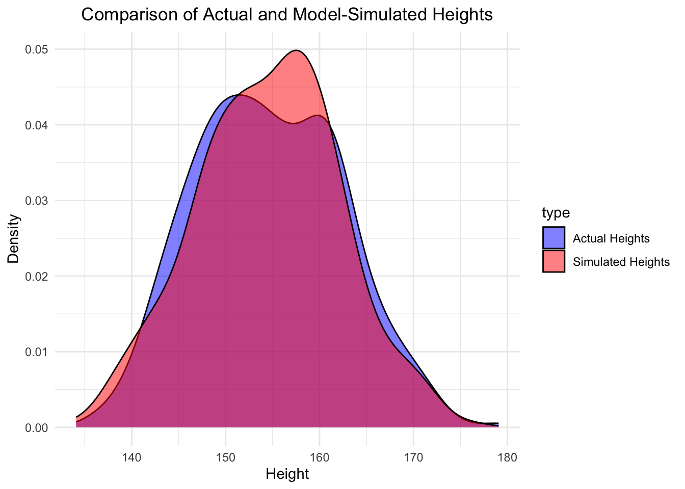
One can repeat the simulation and see how the distributions changes to get a feeling for the variability of the model/data.
2.4 Exercises
[E] Easy, [M] Medium, [H] Hard
(Some) solutions to exercises can be found in the git-repo here.
2.4.1 [E] Exercise 1
Use the Swiss body heights data to determine
- the 95% “Vertrauensintervall” for \(\mu\) and
- calculate the standard deviation of the heights from \(21,873\) Swiss people.
- Read the definition of the confidence interval in the footer of the table and explain why this is correct.
2.4.2 [E] Exercise 2
Why do we not need a hypothesis test to know that the population mean of body heights is not zero? Give 2 reasons.
2.4.3 [H] Exercise 3
Verify analytically that the Residual standard error is identical with
the sample standard deviation of the heights in the simple mean model above.
2.4.4 [M] Exercise 4
Repeat the Bayesian and Frequentist estimation of the simple model using a different data set about chicken weights, which is included in R.
- Set useful priors for the mean and standard deviation of the model for the Bayesian and the frequentist version considering your a priori knowledge about chicken weights.
2.4.5 [M] Exercise 5
- Try to understand/verify the code in the addendum below.
- Change the parameters \(\mu = (\mu_X, \mu_Y)\) and \(\Sigma\) of the bivariate normal distribution and see how the 3D plot changes.
- Plot the scatter plot of the \(X\) and \(Y\) values and compare it to the 3D plot. Does this make sense?
- Why is the scatter plot elliptical?
2.4.6 [M] Exercise 6
Independence of two random variables \(X\) and \(Y\) implies that the correlation between them is zero. A correlation of zero does not necessarily imply independence.
- Verify this counterexample: For example, suppose the random variable \(X\) is symmetrically distributed about zero, and \(Y = X^2\). Then \(\mathit{Y}\) is completely determined by \(X\), so that \(\mathit{X}\) and \(\mathit{Y}\) are perfectly dependent, but their correlation is zero.
2.4.7 [H] Exercise 7
Go to the section about the bivariate normal distribution below.
- How do you get the correlation matrix from the covariance matrix (\(\Sigma\))? \[ \Sigma = \begin{bmatrix} 0.75 & 0.5 \\ 0.5 & 0.75 \end{bmatrix} \] Hint: For the bivariate normal distribution, the correlation matrix is defined here.
2.5 Addendum
2.5.1 The bivariate normal distribution
As a refresher, you can look into the old QM1 script and read the chapter “4.7 Gemeinsame Verteilungen”. Maybe this video also helps.
The bivariate normal distribution is a generalization of the normal distribution to two dimensions. Now, we look at the distribution of two random variables \(X\) and \(Y\) at the same time.
Instead of one Gaussian curve, we have a 3D curve. This curve defines how plausible different combinations of \(X\) and \(Y\) are.
Single points (like (3,6)) still have probability zero, because now the volume over a single point (\(x\), \(y\)) is zero. The probability of a certain area is now the volume under the curve compared to the area under the density curve in the one-dimensional case.
Example: The following plot shows the density of a bivariate normal distribution of two variables \(X\) and \(Y\) with \(\mu_X = 0\), \(\mu_Y = 0\), \(\sigma_X = 1\), \(\sigma_Y = 1\) and \(\rho = \frac{2}{3}\).
Below is the correlation matrix of the bivariate normal distribution.
##           [,1]      [,2]
## [1,] 1.0000000 0.6666667
## [2,] 0.6666667 1.0000000
If you move the plot around with your mouse, you see that there is a positive correlation between \(X\) and \(Y\) (\(\rho = \frac{2}{3}\)). This means that if \(X\) is above its mean, \(Y\) is also more likely to be above its mean. The variances of \(X\) and \(Y\) are both \(1\). That means, that if you cut through the plot in \(X=0\) or \(Y=0\), you see the same form of normal distribution. If you look at it from above, we have highlighted the section on the surface over the area \(X \in [0.5, 2]\) and \(Y \in [0.5, 2]\). The volume over this area under the density curve is the probability of this area: \(P(X \in [0.5, 2] \text{ and } Y \in [0.5, 2])\)
Calculate this probability with R:
# Load the mvtnorm package
library(mvtnorm)

# Define the parameters of the bivariate normal distribution
mu <- c(0, 0)                       # Mean
sigma <- matrix(c(0.75, 0.5, 0.5, 0.75), ncol = 2) # Covariance matrix

# Define the bounds of the square
highlight_x <- c(0.5, 2)
highlight_y <- c(0.5, 2)
# Calculate the probability using pmvnorm
pmvnorm(
  lower = c(highlight_x[1], highlight_y[1]),
  upper = c(highlight_x[2], highlight_y[2]),
  mean = mu,
  sigma = sigma
)
## [1] 0.1526031
## attr(,"error")
## [1] 1e-15
## attr(,"msg")
## [1] "Normal Completion"Since we do not believe everything we are told, we rather check via simulation, if \(0.1526\) is a plausible value for the probability:
# Load necessary library
library(MASS)

# Define the parameters of the bivariate normal distribution
mu <- c(0, 0)                       # Mean
sigma <- matrix(c(0.75, 0.5, 0.5, 0.75), ncol = 2) # Covariance matrix
cov2cor(sigma)  # Convert covariance matrix to correlation matrix
## [,1] [,2]
## [1,] 1.0000000 0.6666667
## [2,] 0.6666667 1.0000000# Define the bounds of the square
highlight_x <- c(0.5, 2)
highlight_y <- c(0.5, 2)
# Number of simulations
n_sim <- 10^4
set.seed(343434)
# Simulate bivariate normal samples
samples <- mvrnorm(n = n_sim, mu = mu, Sigma = sigma)
# Count how many samples fall within the square
inside_square <- sum(
samples[, 1] >= highlight_x[1] & samples[, 1] <= highlight_x[2] &
samples[, 2] >= highlight_y[1] & samples[, 2] <= highlight_y[2]
)
# Estimate the probability
inside_square / n_sim## [1] 0.1557Looks good.
2.6 Sample exam questions for this chapter (in German since exam is in German)
2.6.1 Question 1
Welche der folgenden Aussage(n) hinsichtlich Prediction und Explanation im Kontext statistischer Modellierung ist/sind korrekt?
- Prediction models, die gut funktionieren, lassen im Allgemeinen auch Rückschlüsse auf die zugrunde liegenden kausalen Zusammenhänge zu.
- Prediction models fokussieren sich auf die Güte der Prognose für neue Daten, nicht auf das Verständnis kausaler Beziehungen.
- Explanatory models benötigen eine gute theoretische Fundierung, um kausale Zusammenhänge zwischen Variablen testen zu können.
- Ein Beispiel für ein Explanatory model ist die Klassifikation von Bildern mittels neuronaler Netzwerke.
2.6.2 Question 2
Welche Aussage(n) bezüglich Bayes’scher statistischer Modellierung ist/sind korrekt?
- Bayes’sche Modelle sind nur für kleine Stichproben geeignet, da sie bei großen Datenmengen instabil werden.
- Die Prior-Verteilungen der Parameter beeinflussen die Posterior-Verteilungen der Parameter in der Regel kaum.
- Aus Bayes Modellierung erhält man in erster Linie Punktschätzungen der Parameter.
- Ist der \(p\)-Wert bei einer Hypothese \(H_0\) kleiner als \(0.05\), so ist die Hypothese \(H_0\) falsch.
2.6.3 Question 3
Wir gehen (wie in der Vorlesung) von einem simplen Mittelwert-Modell für Körpergrößen aus.
Welche der folgenden Aussage(n) ist/sind korrekt?
- Die posterioren Verteilungen von \(\mu\) und \(\sigma\) sind stochastisch unabhängig.
- Man ist sich a priori zu (ca.) 95% sicher, dass \(\mu\) im Bereich \([171.1-20, 171.1+20]\) liegt.
- Gäbe es noch eine dritte Variable - z.B. geographische Region - die sowohl \(\mu\) als auch \(\sigma\) beeinflusst, so wäre die Verteilung von \(\mu\) und \(\sigma\) nicht mehr stochastisch unabhängig.
- Je größer die sample size, desto weniger spielen die Priors eine Rolle und desto ähnlicher sind sich die Resultate der Bayes’schen und Frequentistischen Modellierung.